---

Overview

Model Complex Data Sets Fast and Easy

What once could take days of tedious work now takes minutes, with a much more powerful result.

Find Optimum Equations to Describe Empirical Data

TableCurve 3D® gives scientists and engineers the power to find the ideal model for even the most complex data, including equations that might never have been considered. TableCurve 3D’s built-in equation set includes a wide array of linear and nonlinear models for any application:

• Linear equations
• Polynominal and rational functions
• Logrithmic and exponential functions
• Nonlinear peak functions
• Nonlinear transition functions
• Nonlinear exponential and power equations
• User-defined functions (up to 15)

TableCurve 3D’s state-of-the-art surface fitting includes capabilities not found in other software packages:

• In addition to standard least squares minimization, TableCurve 3D’s non-linear engine is capable of three different robust estimations: least absolute deviation, Lorentzian minimization and Pearson VII Limit minimization.
• Option to change the maximum number of terms permitted when fitting linear equations (minimum 3; maximum 11)
• On systems that support multi-threading, TableCurve 3D’s Background Thread Processing option allows fitting to occur without any form of user input
• Option to set the default term significance anywhere from 1 to 15.

Automation Takes The Trial And Error Out Of Curve Fitting

Using its selective subset procedure, TableCurve 3D will fit 36,000 of the over 450 million built-in equations or just the ones you need – instantly. With TableCurve 3D, a single mouse click is all it takes to start the automated curve fitting process – there is no set up required! You can even enter your own specialty models to be fit and ranked along with the built-in equations. TableCurve saves you precious time because it takes the endless trial and error out of curve fitting.

User-Defined Fit Functions

Up to 15 user-defined equations can be entered and ranked along with the built-in equations. These specialized models can contain most mathematical constructs, including special functions, series convergence and conditional statements, differentiations, integrations and parameter constraints. TableCurve 3D even offers the option of graphically adjusting equation parameters to assure convergence for the fit of user-defined models. Unlike most surface fitting programs, TableCurve 3D’s user-defined functions are compiled so they can be fitted at nearly the speed of the built-in equations. For maximum flexibility, TableCurve 3D gives you the option to save your functions as individual files, in libraries or both.

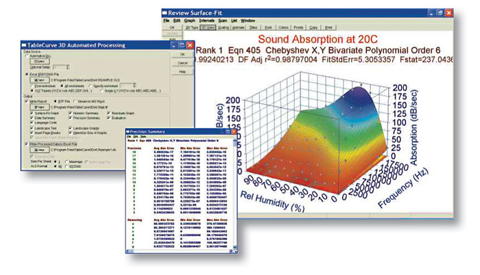
Visually Discover the Best Equation to Model your Data: Graphically Review Surface Fit Results

Once your XYZ data have been fit, TableCurve 3D automatically sorts and plots the fitted equations by the statistical criteria you select (r2, DOF adjusted r2, Fit Standard Error or the F Statistic). Graphically review the fitted results as you scroll through the equation list. A 3D residuals graph as well as parameter output are generated for each fitted equation. Add confidence or prediction intervals to the graph to detect outliers in your data. You can also automatically display a 2D contour plot on the top and bottom of the surface fit graph to get another view of your data. Data, statistical and numeric summaries are also available from within the Review Surface Fit window so you can further analyze fit results.

The Best Fit

Viewing a surface fit from all angles is imperative in determining whether or not a given fit is accurate. Using a simple interface, TableCurve 3D lets you view a graph from any angle. It will even animate the graph automatically in a specified XY and/or Z angle sequence. Just sit back and observe every nuance within the fit. TableCurve 3D gives you all of the tools you need to discover the model that best meets your requirements for the ideal fit.

Flexible Output Options

Output TableCurve 3D’s publication-quality graphs in black and white or color, portrait or landscape. You can also produce files containing data and equations in Lotus, Excel, ASCII, Quattro Pro and SigmaPlot formats. TableCurve 3D can speed up your programming by generating actual function code and test routines for all fitted equations in FORTRAN, C, Basic and Pascal.

All This Power – and Still Easy to Use!

TableCurve 3D takes full advantage of the Windows graphical user interface to simplify every aspect of operation – from data import to output of results. Import data from many popular file formats including SigmaPlot, Excel, Lotus, SPSS and ASCII. Once your data are in the TableCurve editor, start the automatic fitting process with a single mouse click. Choose to fit all equations, select a group of equations or create a custom equation set. All equations are readily available from the Toolbar or TableCurve’s Process Menu. You can even set up TableCurve 3D to begin fitting the moment data are imported or modified with Background Thread Processing Fitting. Users consistently comment that – out of the box, without reading the instructions – TableCurve is highly intuitive, easy-to-use and remarkably simple to learn.

---

General Features

The product features for PeakFit are detailed below in the following categories:

Data Input

• ASCII
• Excel®
• Lotus 123®
• Quattro Pro®Windows®
• SigmaPlot®
• AIA Chromatography
• dBase ® III+, IV
• DIF
• ASCII and Spreadsheet – like Editors
• Averaging Digital Filter

Data Preparation

• Gaussian Deconvolution to remove Spectrophotometer Instrument Response smearing
• Exponential Deconvolution to remove Chromatographic Detector Response smearing
• Smoothing (Savitsky Golay, FFT Filter, Loess, Gaussian Convolution)
• Real – time FFT/Time Domain Graphical Editor
• Dual Graph Data Sectioning with Graphical data point exclusion
• Non – Parametric Digital Filter to Filter or augment data
• Compare with Reference
• Subtract Baseline Imported from File
• Data Transforms
• Area Normalization
• Inspect Second and Fourth Derivatives
• Data Weighting

Peak Autoplacement

• Automatic by Local Maxima and Residuals
• Automatic by Second Derivatives
• Automatic by Deconvolved Local Maxima
• Graphical Placement and Adjustments
• Manual Parameter Adjustments
• Share and Lock Parameters
• Constant or V ariable Widths and/or Shape in a single step

Non-Linear Curve Fitting

• Marquardt – Levenburg Algorithm
• 83 built-in nonlinear peak models
• Least – Squares and 3 Robust (Maximum Likelihood) methods
• Up to 100 Peaks and 1000 Parameters
• Intelligent Constraints to insure Fit Integrity
• Sparse Curvature Matrix for Faster Fitting
• Both Numeric and Graphical Fitting Options
• Zoom – in or Toggle Points during Fitting

Output and Export Options

• File Export with full Generated Data: Lotus 123, Excel, Quattro Pro Windows, SigmaPlot, and ASCII
• Graphs to clipboard or file in BMP or WMF formats
• All Numeric data in Graph to Clipboard in Spreadsheet Format

Automation

Automation Code Generation

• FORTRAN 77, FORTRAN 90, C, C-80 bit, QBasic and Pascal
• Function code or function code with full test routines
• Available for all built-in equations

TableCurve 3D Surface Fitting Features

3D surface fitting features in TableCurve 3D are listed below:

Technical Specifications

• 453,697,490 built-in equations
• 243 polynomials, including 18 Taylor series polynomials, 36 Chebyshev polynomials, 13 Fourier simple and true bivariate models, 9 Cosine Series models, 9 Sigmoid Series models
• 260 rationals, including 4 rationals with Taylor series numerators and denominators and 40 Chebyshev rationals
• 453,696,714 selective subset mixed basis function linear equations, of which up to 36,582 will be selected within a given fit
• 72 3D nonlinear peak equations
• 72 3D nonlinear transition equations
• 24 3D nonlinear exponential and power equations
• 4 robust plane equations
• Rapid searching, sorting, and filtering of equations
• User customizable equation sets
• Full control of fit process, including goodness of fit criteria, minimization and other options
• Robust plane fitting option
• Three robust fitting methods available for all nonlinear equations and user functions

User-Defined Functions (UDFs)

• UDF editor with push-button help for inserting functions
• UDFs automatically compiled for speed
• Up to 15 UDFs can be fit at one time, each with up to 10 adjustable parameters
• Graphical UDF adjustment procedure for refining starting estimates
• UDFs can be saved as libraries

Non-Parametric Fitting

• Algorithms for gridded data include B-Spline, Bicubic+Akima, Akima III, B-Spl Var knots, NURBS
• Algorithms for scattered data include Akima I, Akima II, Preusser, Renka I,Renka II, Renka III, Watson, Loess
• Fill Sparse Grid option that uses scattered data interpolation algorithms to complete a sparse or incomplete grid
• Interpolate Uniform grid option that uses scattered data algorithms to generate a uniform grid of estimated values

Surface-Fit Analysis and Output Numerical

• Evaluation option with automated table generation, includes function, derivatives, roots and cumulative volume
• Full numeric and statistical summary, including coefficients, standard error, confidence limits, ANOVA, goodness of fit, measured function minima and maxima
• Data summary with predicted values, residuals and confidence/prediction limits
• Precision summary and term significance analysis
• Quick Evaluation option for estimation at a point, minimum, maximum
• Save Quick Evaluation and Evaluation across all sessions
• Five levels of perspective for 3D viewing with full angular control of light source illumination
• Confidence/prediction intervals (90%, 95%, 99%, 99.9%, 99.99%)
• Intellimouse rotation of 3D view angles
• Inspect any of the five first or second order partial derivatives

Graphical

• Surface-fit graph with customizable layout, backplanes, labels, grids, scaling, points, font, titles and resolution
• All customizations rendered in real time
• Fourteen types of gradient plots, including one each for Excel, Lotus and Quattro palettes
• Four types of shaded plots with full angular control of light source illumination
• Gradient and shaded plots use up to 32 colors
• Mesh resolution up to 120×120
• Contour plots can be added automatically
• Full animation of fitted surfaces
• Adjustable cache size and compression method for surface-fit graphs
• 3D Residuals graphs

---

System Requirements

Below are the minimum requirements to run TableCurve:

Hardware

• 486 Processor or higher
• 16 MB RAM required (32 MB or more recommended)
• 10MB hard disk space

Software

• Windows 10, 8.x,  7, Windows Vista, 95, 98, NT and XP (32 bit)