Advisory Statistics For Non-Statisticians
Adalta è Rivenditore Unico per l’Italia di Grafiti SigmaStat. Richiesta quotazione…
A cosa serve SigmaSTAT
SigmaSTAT vi aiuta ad analizzare i dati con sicurezza e a visualizzare i risultati con facilità
SigmaStat è un pacchetto software statistico facile da usare “wizard-based” ovvero fornito di una sistema di analisi con procedura assistita.
E’ progettato per guidare gli utenti in ogni fase dell’analisi ed eseguire potenti analisi statistiche senza essere esperti di statistica.
SigmaStat è stato concepito per il settore della ricerca medica e delle scienze della vita, ma può essere un prodotto prezioso per gli scienziati di molti settori.
SigmaStat vi guida passo dopo passo nell’analisi e vi permette di:
- Utilizzare il metodo statistico corretto per analizzare i vostri dati
- Evitare il rischio di errori statistici
- Interpretare correttamente i risultati
- Generare una visualizzazione appropriata e una pubblicazione professionale
Caratteristiche dell’ultima versione di SigmaSTAT
In 2007, SigmaSTAT’s functions and features were integrated into SigmaPlot starting at version 11.
However, on February 1, 2016, SigmaStat 4.0 was released and is now available as a standalone product.
Below are the many improvements to the statistical analysis functions in SigmaSTAT:
- Principal Components Analysis (PCA) – Principal component analysis is a technique for reducing the complexity of high-dimensional data by approximating the data with fewer dimensions.
- Analysis of Covariance (ANCOVA) – Analysis of Covariance is an extension of ANOVA (Analysis of Variance) obtained by specifying one or more covariates as additional variables in the model.
- Cox Regression – This includes the proportional hazards model with stratification to study the impact of potential risk factors on the survival time of a population. The input data can be categorical.
- One-Sample T-test – Tests the hypothesis that the mean of a population equals a specified value.
- Odds Ratio and Relative Risk tests – Both tests the hypothesis that a treatment has no effect on the rate of occurrence of some specified event in a population. Odds Ratio is used in retrospective studies to determine the treatment effect after the event has been observed. Relative Risk is used in prospective studies where the treatment and control groups have been chosen before the event occurs.
- Shapiro-Wilk Normality test – A more accurate test than Kolmogorov-Smirnov for assessing the normality of sampled data. Used in assumption checking for many statistical tests, but can also be used directly on worksheet data.
- New Result Graph – ANOVA Profile Plots: Used to analyze the main effects and higher-order interactions of factors in a multi-factor ANOVA design by comparing averages of the least square means.
- New Probability Transforms – Thirty four new functions have been added to SigmaStat’s Transform language for calculating probabilities and scores associated with distributions that arise in many fields of study.
- New Interface Change – Nonlinear Regression: An easy to use wizard interface and more detailed reports.
- New Interface Change – Quick Transforms: An easier way of performing computations in the worksheet.
- New Interface Change – New User Interface: Allows the user to work more easily with Excel worksheets.
- Yates correction added to the Mann-Whitney test – Yates correction for continuity, or Yates chi-square test is used when testing for independence in a contingency table when assessing whether two samples of observations come from the same distribution.
- Improved Error Messaging – Improved error messages have added information when assumption checking for ANOVA has failed.
- Deming Regression – Deming regression allows for errors in both X and Y variables – a technique for method comparison where the X data is from one method and the y data the other. The Deming regression method basically extends the normal linear regression, where the X values are considered to be error-free, to the case where both X and Y (both methods) have error. Hypotheses can then be tested, slope different from 1.0 for example, to determine if the methods are the same. For example, it might be used to compare two instruments designed to measure the same substance or to compare two algorithmic methods of detecting tumors in images. The graph compares the two methods to determine if they are different or the same. A report gives statistical results.

- Akaike Information Criterion (AICc) – The Akaike Information Criterion is now available in nonlinear regression reports. It is a goodness of fit criterion that also accounts for the number of parameters in the equation. It also is valid for non-nested equations that occur, for example, in enzyme kinetics analyses.
- New Probability Functions for Nonlinear Regression – A total of 24 probability functions have been added to the curve fit library. Automatic initial parameter estimate equations have been created for each.
- Nonlinear Regression Weighting – There are now seven different weighting functions built into each nonlinear regression equation (3D are slightly different). These functions are reciprocal y, reciprocal y squared, reciprocal x, reciprocal x squared, reciprocal predicteds, reciprocal predicteds squared and Cauchy. The iteratively reweighted least squares algorithm is used to allow the weights to change during each nonlinear regression iteration.
- Multiple Comparison Test Improvements – Two important improvements have been made. P values for the results of nonparametric ANOVA have been added. These did not exist before. Also, multiple comparison P values were limited to discrete choices (0.05, 0.01, etc.). This limitation no longer exists and any valid P value may be used.
Major New Statistical Tests
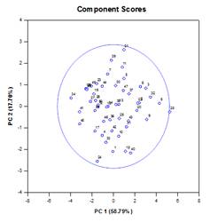
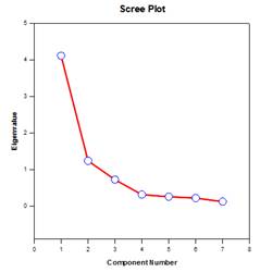
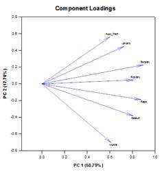
Principal Components Analysis (PCA) – Principal component analysis is a technique for reducing the complexity of high-dimensional data by approximating the data with fewer dimensions. Each new dimension is called a principal component and represents a linear combination of the original variables. The first principal component accounts for as much variation in the data as possible. Each subsequent principal component accounts for as much of the remaining variation as possible and is orthogonal to all of the previous principal components.
You can examine principal components to understand the sources of variation in your data. You can also use them in forming predictive models. If most of the variation in your data exists in a low-dimensional subset, you might be able to model your response variable in terms of the principal components. You can use principal components to reduce the number of variables in regression, clustering, and other statistical techniques. The primary goal of Principal Components Analysis is to explain the sources of variability in the data and to represent the data with fewer variables while preserving most of the total variance.
Examples of Principal Components Graphs:
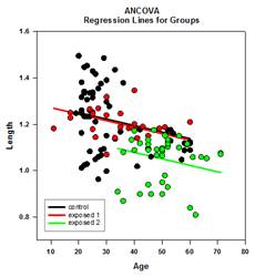
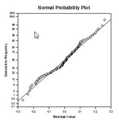
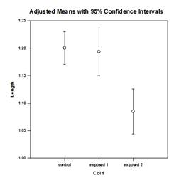
Analysis of Covariance (ANCOVA) – Analysis of Covariance is an extension of ANOVA obtained by specifying one or more covariates as additional variables in the model. If you arrange ANCOVA data in a SigmaPlot worksheet using the indexed data format, one column will represent the factor and one column will represent the dependent variable (the observations) as in an ANOVA design. In addition, you will have one column for each covariate.
Examples of ANCOVA Graphs:

New Statistical Features
Multiple Comparison Improvements – A significant improvement in multiple comparison P value computation has been made. The following multiple comparison procedures, Tukey (non-parametric tests), SNK (non-parametric tests), Dunnett’s, Dunn’s (non-parametric only), and Duncan did not compute p-values analytically, but instead used lookup tables of critical values for a particular distribution to determine, using interpolation if necessary, whether a computed test statistic represented a significant difference in the group means. Thus, p-values were not reported for these tests, but only the conclusion of whether a significant difference existed or not. A major problem with this approach is that the lookup tables are only available for two significance levels, .05 and .01. Another problem is that many customers want to know the p-values. For SigmaPlot, algorithms have been coded to compute the distributions for the test statistics for all post-hoc procedures, making the lookup tables obsolete. As a result, adjusted p-values for all post-hoc procedures are now placed in the report. Also, there is no longer any need to restrict the significance level of multiple comparisons to .05 or .01. Instead, the significance level of multiple comparisons will be the same as the significance level of the main (omnibus) test. There is no limitation on this p value – any valid value may be used.
Akaike Information Criterion (AICc) – The Akaike Information Criterion has been addedto the Regression Wizard and Dynamic Fit Wizard reports and the Report Options dialog. It provides a method for measuring the relative performance in fitting a regression model to a given set of data. Founded on the concept of information entropy, the criterion offers a relative measure of the information lost in using a model to describe the data.
More specifically, it gives a tradeoff between maximizing the likelihood for the estimated model (the same as minimizing the residual sum of squares if the data is normally distributed) and keeping the number of free parameters in the model to a minimum, reducing its complexity. Although goodness-of-fit is almost always improved by adding more parameters, overfitting will increase the sensitivity of the model to changes in the input data and can ruin its predictive capability.
The basic reason for using AIC is as a guide to model selection. In practice, it is computed for a set of candidate models and a given data set. The model with the smallest AIC value is selected as the model in the set which best represents the “true” model, or the model that minimizes the information loss, which is what AIC is designed to estimate.
After the model with the minimum AIC has been determined, a relative likelihood can also be computed for each of the other candidate models to measure the probability of reducing the information loss relative to the model with the minimum AIC. The relative likelihood can assist the investigator in deciding whether more than one model in the set should be kept for further consideration.
The computation of AIC is based on the following general formula obtained by Akaike1


where is the number of free parameters in the model and is the maximized value of the likelihood function for the estimated model.


When the sample size of the data is small relative to the number of parameters (some authors say when is not more than a few times larger than ), AIC will not perform as well to protect against overfitting. In this case, there is a corrected version of AIC given by:

It is seen that AICc imposes a greater penalty than AIC when there are extra parameters. Most authors seem to agree that AICc should be used instead of AIC in all situations.
Probability Fit Functions – 24 new probability fit functions have been added to the fit library standard.jfl. These functions and some equations and graph shapes are shown below:

As an example, the fit file for the Lognormal Density function contains the equation for the lognormal density lognormden(x,a,b), equations for automatic initial parameter estimation and the seven new weighting functions.
[Variables]
x = col(1)
y = col(2)
reciprocal_y = 1/abs(y)
reciprocal_ysquare = 1/y^2
reciprocal_x = 1/abs(x)
reciprocal_xsquare = 1/x^2
reciprocal_pred = 1/abs(f)
reciprocal_predsqr = 1/f^2
weight_Cauchy = 1/(1+4*(y-f)^2)
‘Automatic Initial Parameter Estimate Functions
trap(q,r)=.5*total(({0,q}+{q,0})[data(2,size(q))]*diff(r)[data(2,size(r))])
s=sort(complex(x,y),x)
u = subblock(s,1,1,1, size(x))
v = subblock(s,2,1,2, size(y))
meanest = trap(u*v,u)
varest=trap((u-meanest)^2*v,u)
p = 1+varest/meanest^2
[Parameters]
a= if(meanest > 0, ln(meanest/sqrt(p)), 0)
b= if(p >= 1, sqrt(ln(p)), 1)
[Equation]
f=lognormden(x,a,b)
fit f to y
”fit f to y with weight reciprocal_y
”fit f to y with weight reciprocal_ysquare
”fit f to y with weight reciprocal_x
”fit f to y with weight reciprocal_xsquare
”fit f to y with weight reciprocal_pred
”fit f to y with weight reciprocal_predsqr
”fit f to y with weight weight_Cauchy
[Constraints]
b>0
[Options]
tolerance=1e-010
stepsize=1
iterations=200
Weight Functions in Nonlinear Regression – SigmaPlot equation items sometimes use a weight variable for the purpose of assigning a weight to each observation (or response) in a regression data set. The weight for an observation measures its uncertainty relative to the probability distribution from which it’s sampled. A larger weight indicates an observation which varies little from the true mean of its distribution while a smaller weight refers to an observation that is sampled more from the tail of its distribution.
Under the statistical assumptions for estimating the parameters of a fit model using the least squares approach, the weights are, up to a scale factor, equal to the reciprocal of the population variances of the (Gaussian) distributions from which the observations are sampled. Here, we define a residual, sometimes called a raw residual, to be the difference between an observation and the predicted value (the value of the fit model) at a given value of the independent variable(s). If the variances of the observations are not all the same (heteroscedasticity), then a weight variable is needed and the weighted least squaresproblem of minimizing the weighted sum of squares of the residuals is solved to find the best-fit parameters.
Our new feature will allow the user to define a weight variable as a function of the parameters contained in the fit model. Seven predefined weight functions have been added to each fit function (3D functions are slightly different). The seven shown below are 1/y, 1/y2, 1/x, 1/x2, 1/predicted, 1/predicteds2 and Cauchy.

One application of this more general adaptive weighting is in situations where the variances of the observations cannot be determined prior to performing the fit. For example, if all observations are Poisson distributed, then the population means, which are what the predicted values are estimating, equal to the population variances. Although the least squares approach for estimating parameters is designed for normally distributed data, other distributions are sometimes used with least squares when other methods are unavailable. In the case of Poisson data, we need to define the weight variable as the reciprocal of the predicted values. This procedure is sometimes referred to as “weighting by predicted values”.
Another application of adaptive weighting is to obtain robust procedures for estimating parameters that mitigate the effects of outliers. Occasionally, there may be a few observations in a data set that are sampled from the tail of their distributions with small probability, or there are a few observations that are sampled from distributions that deviate slightly from the normality assumption used in least squares estimation and thus contaminate the data set. These aberrant observations, called outliers in the response variable, can have a significant impact on the fit results because they have relatively large (raw or weighted) residuals and thus inflate the sum of squares that is being minimized.
One way to mitigate the effects of outliers is to use a weight variable that is a function of the residuals (and hence, also a function of the parameters), where the weight assigned to an observation is inversely related to the size of the residual. The definition of what weighting function to use depends upon assumptions about the distributions of observations (assuming they are not normal) and a scheme for deciding what size of residual to tolerate. The Cauchy weighting function is defined in terms of the residuals, y-f where y is the dependent variable value and f is the fitting function, and can be used for minimizing the effect of outliers.
weight_Cauchy = 1/(1+4*(y-f)^2)
The parameter estimation algorithm we use for adaptive weighting, iteratively reweighted least squares (IRLS), is based on solving a sequence of constant-weighted least squares problems where each sub-problem is solved using our current implementation of the Levenberg-Marquardt algorithm. This process begins by evaluating the weights using the initial parameter values and then minimizing the sum of squares with these fixed weights. The best-fit parameters are then used to re-evaluate the weights.
With the new weight values, the above process of minimizing the sum of squares is repeated. We continue in this fashion until convergence is achieved. The criterion used for convergence is that the relative error between the square root of the sum of the weighted residuals for the current parameter values and the square root of the sum of weighted residuals for the parameter values of the previous iteration is less than the tolerance value set in the equation item. As with other estimation procedures, convergence is not guaranteed.
Statistical Features
Analysis of Variance and Covariance
- Independent and paired two sample t-tests, one-sample t-test
- One, two, and three way ANOVA
- One and two way repeated measures and mixed ANOVA
- One way ANCOVA with multiple covariates
Nonparametric Tests
- One-sample signed rank test
- Mann-Whitney rank sum test
- Wilcoxon signed rank test
- Kruskal-Wallis ANOVA on ranks
- Friedman repeated measures ANOVA
Correlation
- Pearson product moment
- Spearman rank order
Descriptive Statistics
- Sample mean, standard deviation, standard error of mean, median, percentiles, sum and sum of squares, skewness, kurtosis, confidence interval for the mean, range, maximum and minimum values, normality tests, sample size, missing value content
Principal Components Analysis
- Covariance or correlation matrix analysis, multiple methods of component selection
Power and Sample Size in Experimental Design
- T-tests, ANOVA, proportions, chi-square and correlation
ANOVA Multiple Comparison Procedures
- Holm-Sidak
- Tukey
- Duncan’s Multiple Range
- Fisher LSD
- Student-Newmann-Keuls
- Bonferroni t-test
- Dunnett’s t-test
- Dunn’s test
Statistical Transforms
- Stack data
- Index and Un-index data for one or two factor variables
- Center, standardize, and rank data
- Apply simple transforms to data using arithmetic operations and basic numerical functions
- Create dummy variables with either reference coding or effects coding
- Create sequences of random numbers that are uniform or normally distributed
- Filter data from worksheet columns using a key column
Regression
- Linear and multiple linear
- Polynomial for a specific order and model comparisons for several orders
- Stepwise, forward and backward
- Best subsets
- Multiple logistic
- Deming
- Nonlinear,using built-in and user-defined models
Rates and Proportions
- Chi-Square analysis of contingency tables
- McNemar’s test
- Fisher exact test
- Z-test
- Odds Ratio
- Relative Risk
Survival Analysis
- Kaplan-Meier, including single group, LogRank, and Gehen-Breslow
- Cox Regression, including proportional hazards and stratified models
Normality
- Shapiro-Wilk
- Kolmogorov-Smirnov with Lilliefors correction
Equal Variance
- Brown-Forsythe test for ANOVA analysis
- Spearman rank correlation test for regression analysis
Test Options
- Check test assumptions like normality and equal variance that, if violated, may prompt the user to choose an alternate test
- Criterion options that change the way the analysis for a test is performed
- Options for running multiple comparison tests depending on the significance of main test effects
- Options for placing residuals, confidence intervals, predicted values, and weights in the worksheet
- Additional statistics and diagnostics in reports that explore your data and enhance the results, including outlier detection, multicollinearity, retrospective power and residual analysis
- Result graph options for scaling, error bars and color.
Requisiti di sistema di SigmaSTAT
Hardware
- 2 GHz 32-bit (x86) or 64-bit (x64) Processor
- 2 GB of System Memory for 32-bit (x86)
- 4 GB of System Memory for 64-bit (x64)
- 200 MB of Available Hard Disk Space
- CD-ROM Drive
- 800×600 SVGA/256 Color Display or better
- Internet Explorer Version 8 or better
Software
- Windows XP, Windows Vista, Windows 7, Windows 8.x, Windows 10; Internet Explorer 8 or higher
- Office 2003 or higher (paste to Powerpoint Slide, Insert Graphs into Word and other macros)